Introduction

Peanut (Arachis hypogaea L.) is a globally important crop valued for its nutritional content and versatility. The Virginia-Carolinas (V-C) region of the United States primarily grows Virginia-type peanuts, characterized by larger pod sizes than the predominant runner-type grown throughout the southeast. Cultivation of Virginia-types benefits from the lightly colored, sandy soil of the coastal V-C to ensure pods retain their distinctive hue and minimize visual blemishes. Virginia-type production also generally requires additional inputs, particularly water and gypsum, to produce larger pods and ensure seeds adequately fill those larger pods (Stalker, 1997). Farmers receive higher contract prices and/or premiums for Virginia-types, currently ~$6/ton over runner-types (USDA NASS, 2025). Farmers also receive premiums for larger seed size, which has many determining factors, but is ultimately limited by pod size.

Farmers first take their trailer to a ‘buying point’ where a sampler (most commonly pneumatic) is used to collect a representative pod sample (approximately 3,600g) from the full load. The sample is then partitioned in half (minimum 1,500g) using a farmers’ stock sample divider with foreign material (FM) and loose shelled kernels (LSKs) are next removed by a purpose built machine followed by hand sorting, if necessary (USDA, 2019). The pre-sizer, initially designed in 1959 (Dickens, 1962) consists of two rotating metal ‘rollers’ separated initially by a spacing of 13.5mm (17/32") which widens to 15.1mm (19/32”) at the ‘step’. The smallest pods fall through the initial opening into the small (blue or "No. 1") pan, medium sized pods fall through the second opening into the medium (white or "Fancy") pan and the largest pods fall off the end of the rollers into the large (red or "Jumbo") pan.

The grader is required to take an initial weight of the sample, feed pods into the roller at a reasonable rate, remove the corresponding pans for the three categories, record their weights individually, calculate the percent weight of each pan of the full sample, and keep each sample separate so they can be shelled appropriately. Therefore, the system is partially quantitative with limited utility and labor-intensive. It is also error prone as pods can ‘ride’ on top of each other and fall into a larger bin than they should. Additionally, the rollers are manually set using common drill bits and commonly become wider or narrower than intended without the operator noticing. Larger peanuts will split when shelled into smaller compartments while smaller peanuts will not shell properly in larger compartments.

Virginia-type loads with greater than 40% Fancy pods are generally considered more valuable. Percentage of Fancy pods is determined by subtracting the weight of the small, blue pan from the weight of the cleaned sample, then dividing by the weight of the cleaned sample (USDA, 2019).

To be classified as a Virginia-type, the crop must have at least 40% of pods ‘graded’ as Fancy or Jumbo (USDA, 2019; Isleib et al. 2006). After measuring foreign material in the farmers’ stock, a sample of cleaned pods is then shelled to determine the percentage of various sound and damaged kernels, in addition to the presence/absence of Aspergillus flavus mold, among other grade factors (USDA, 2019). The entire process typically takes 30 minutes per sample and ends with a score being assigned to the load, from which a price is determined. In addition to these commercial loads, the same process is carried out in breeding programs to assess the merit of breeding lines for advancement to cultivar status.

While larger pods and seeds are generally preferred by food manufacturers and consumers, and varieties that produce them are readily available, there are three obstacles to their widespread adoption. The first is farmers have no incentive to produce a crop with pods larger than the minimum requirements to classify as a Virginia-type, as there is no premium to do so. This is at least partially due to the current inability to provide a fully quantitative measure of, and therefore reward for, pod size. Secondly, peanut seed is sold per pound and as the seed generally gets larger and heavier with increased pod size, there are fewer seeds per pound. This directly increases planting costs as growers must purchase more pounds of seed to plant a given number of seeds per foot of row length. The recommended seeding rate for Virginia-type peanuts in the VC region is 13-19 seed per meter or row (4-6 seeds per foot of row). This translates roughly to 143,000-200,000 seeds per hectare (58,000-81,000 seeds per acre). This typically requires 141-180 kg of seed per hectare (125-160 pounds of seeds per acre), compared to 123 kg of seed per hectare (110 pounds of seed per acre) for runner type peanuts (Jordan, 2023). If seed could be counted accurately and sold on a count basis it would eliminate this inherent penalty of large-seeded varieties. Third, shellers are often reluctant to change the grates on their peanut shellers. Therefore, large-podded and seeded varieties are often shelled on grates that are too small, resulting in an unacceptably high level of split kernels. Thus, as the system currently exists, the ideal Virginia-type has the smallest and lightest seed that produces the bare minimum pod size to gain classification as a Virginia-type and the largest seed that can comfortably fit through the standard shelling grate.

Recent advances in computer vision offer new opportunities to improve pod grading. Computer models can be ‘trained’ to precisely identify and delineate individual objects in an image or video by generating pixel-level ‘masks’ to outline the object boundaries and differentiate them from one another (Hafiz & Bhat, 2020). ‘Training sets’ of manually annotated images are used to train models which are then validated on ‘validation sets’ the model has not seen, prior to the model’s deployment. Mask Region-based Convolutional Neural Networks (Mask R-CNN) perform this ‘image segmentation’ by using a Region Proposal Network (RPN) to propose bounding boxes from which a mask is predicted by a fully convolutional network (FCN) (He et al., 2017). From the mask, various object parameters can be calculated including object length, width, and area. Mask R-CNN has been used to assess various morphological traits in soybean (Yang et al., 2021), maturity in vined tomato (Afonso et al., 2020), and seed morphology of various crops (Toda et al., 2020).

The objective of this study was to develop and validate a computer vision-based phenotyping platform capable of rapidly and accurately measuring pod width and assigning USDA pod grade categories, providing a more quantitative and efficient alternative to the current mechanical roller system while simultaneously collecting more in-depth pod information.

Materials and Methods

Imaging System

The imaging system consisted of a Luxonis OAK-D camera and Globe Electric 10-inch Selfie LED ring light physically mounted to a K&F Concept camera tripod set to the minimum 55.88cm (22”) height on a solid black background (Figure 1). Despite the OAK-D camera being capable of depth imaging, the resolution was not high enough to differentiate pods and background at such a close distance, so depth information was not used in this study. Direct lighting was initially employed; however, inconsistent shadowing prompted a transition to diffuse lighting, which improved illumination consistency across samples. Shown in Figure 1 is a standard lab bench but if one is unavailable, a black canvas can be used. Included in the background is an ‘ArUco marker,’ the black and white square seen in Figure 1. The ArUco marker is used to convert the number of pixels in the image into a usable unit of measure (in this case mm) as the exact dimensions of the ArUco marker (50mm x 50mm) are known and OpenCV has a built in ArUco recognition library (Garrido-Jurado et al., 2014, Bradski, 2000). Likewise, the color card seen in Figure 1 provides known colors so each image can be corrected to a known and consistent color space, particularly under changing lighting conditions. The camera was attached via USB cable to a standard computer with the Luxonis DepthAI Python API installed to control the OAK-D camera (Luxonis, 2023).

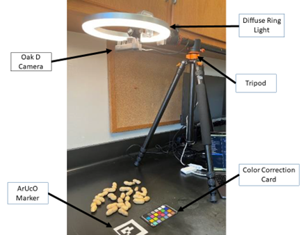
Figure 1. Imaging system setup. A Luxonis OAK-D camera and Globe Electric 10-inch Selfie LED Diffuse Ring Light were mounted to a K&F Concept Camera Tripod set to the minimum height of 55.88cm (22”). Placed under the camera and ring light but on top of the black background are a black and white ArUco marker for determining object size and an multicolored card for color correction.

Mask Region-based Convolutional Neural Networks (Mask R-CNN) Model and Pod Measurement Extraction

The development of a Mask R-CNN model (He et al., 2017) was proposed based on its ability to accurately identify down to the pixel level individual pods. To train this model, 584 images were taken of hundreds of pods of several genotypes representing the full variance of pod size in the North Carolina State University (NCSU) breeding program. Images were taken with varying backgrounds, number of pods per image, and levels of contact between pods (Figure 2). Images were manually labeled using the free version of Hasty.ai (Hasty.ai, 2023) as either pod or background. Labeled images were exported in Common Objects in Context (COCO) format from Hasty.ai (Hasty.ai, 2023). The Mask R-CNN implementation (Abdulla, 2017) was downloaded and adapted for use in TensorFlow 2.5 (Google, 2021) and Google Colab (Google, 2023). Due to time and computation limits on Google Colab, a Dell Precision 7820 Tower PC with two Intel Xeon Silver 4112 2.6GHz CPUs and 112 Gb of memory was upgraded with a NVIDIA GeForce RTX A5000 GPU to complete the training runs.

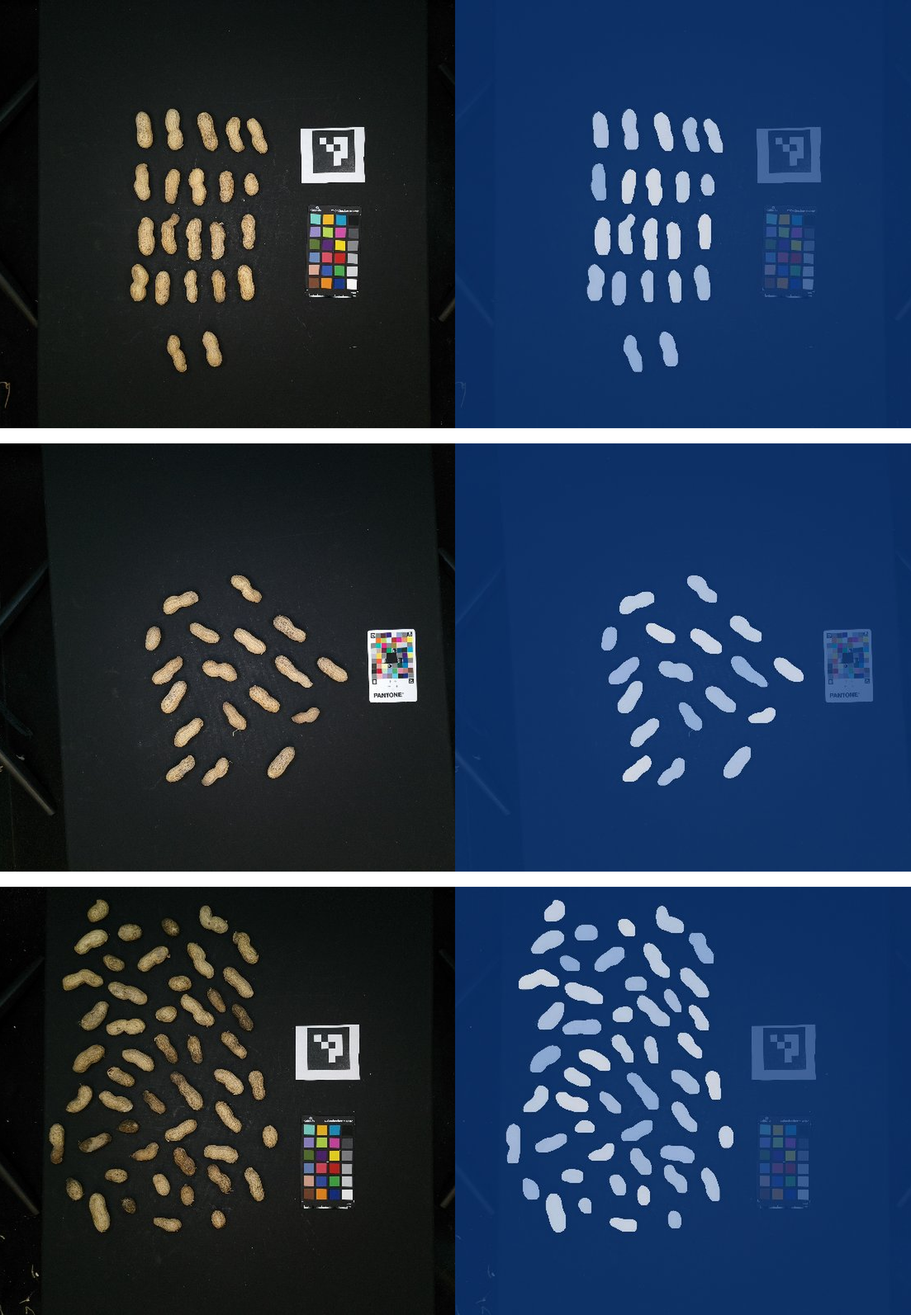
Figure 2. Example input images for the Mask R-CNN model training (left) and their respective instance segmentations masks (right). Individual masks are distinguished by varying shades from blue to white, with each peanut pod rendered in a distinct shade to differentiate overlapping instances. All peanut pods in the input images were manually annotated using the Hasty.ai web-based annotation platform to generate instance segmentation masks, which were used as training data for the model to learn to detect and segment individual peanut pods.

Anaconda (Anaconda, Inc., 2023), the free, open-source distribution of Python and R, was used to create a Python 3.9 environment instance with necessary “dependencies” installed. Anaconda bundles Python with a package manager named “conda” and hundreds of pre-installed libraries and tools creating a user-friendly data science environment, especially for computer vision applications. In software terminology, a “dependency” is an external, pre-built, and mandatory piece of code, often for common features, to save time during code writing. As the Hasty.ai COCO output varied between polygon and run-length encoding (RLE) label format, a Python script was written to convert all RLE formatted sections to polygon format. The TensorFlow Object Detection API guide (Vladimirov, 2021) was used to ensure necessary software was installed and compatible with the hardware being used.

Our model training parameters were set to 50 epochs (50 iterations over the entire training set of 584 images) on an 80/20 training/validation split. This method was used to overfit a model and then select the best version of the model based on validation accuracy after training has finished. Examples of input images and their respective masks can be seen in Figure 2. The best model was chosen based upon the lowest training loss (how well the model performs with images it was trained on) and validation loss (how well the model performs on new images) with loss visualized using TensorBoard (TensorFlow Developers, 2023) as seen in Figure 3. OpenCV (Bradski, 2000), numpy (Harris et al., 2020), and pandas (McKinney, 2011) python packages were used to measure the width of each successfully recognized individual pod and output this information to a .csv file for statistical analysis. OpenCV length, width and area functions were used to extract characteristics from each pod in pixel units. The pixel values were converted to mm using the pixel to mm conversion factor calculated from the ArUco marker. Pod width was then used to determine a pod’s placement in its mechanical grading category (No. 1, Fancy or Jumbo). Excessively large (>23mm) or small (<6mm) widths were considered faulty outputs and discarded. The number of pods the algorithm was allowed to detect per image was capped at 100 for consistency across images. The 100 pods were selected at random. The Mask R-CNN model optimizes a multi-task loss function comprising classification loss, bounding box regression loss, and mask segmentation loss, with the total loss representing the sum of these components across all detected instances (He et al., 2017). Within each epoch, the full training dataset was processed in discrete steps, at each of which the model evaluated its predictions against ground truth annotations and adjusted its weights via backpropagation to minimize the loss function. At the end of each epoch, the model state was saved as a checkpoint, allowing selection of the model that best balanced training loss reduction with validation performance. To test the accuracy of the Mask R-CNN model, three 50-pod samples of 25 genotypes representative of the NCSU breeding program were selected, imaged, and analyzed. After imaging, calculated pod width data was used to place each pod into either the No. 1, Fancy, or Jumbo category. The same pods were then graded using traditional mechanical rollers, which were carefully calibrated before running these samples. Model detection performance was evaluated using precision, recall, F1 score, and mean average precision (mAP) at an IoU threshold of 0.5 (Lin et al., 2014), where precision reflects the proportion of detections that were true pods, recall reflects the proportion of actual pods successfully detected, F1 score represents the harmonic mean of precision and recall, and mAP summarizes detection accuracy across all confidence thresholds. Spearman's correlation coefficient, a monotonic rank-based measure of statistical association, was then used to determine the degree of association between mechanical grade and the Mask R-CNN model (Spearman, 1904).

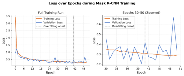
Figure 3. Validation and training loss over 50 steps of Mask R-CNN training (left) and magnification of steps 30-50 of the validation and epoch loss (right). The dashed line represents the onset of model overfitting as there is a marked increase in validation loss (performance on new images) despite continued reductions in training loss (performance on training images). Thus, “checkpoint selection” was necessary to identify the best performing model.

Proof-of-Concept Field Study

A set of 265 inbred genotypes was selected to represent the diversity of the NCSU breeding program. This set included advanced breeding material, released cultivars, and germplasm lines containing wild species introgressions from A. cardenasii.

The trials were grown in two years (2021 and 2022) at three locations, the Upper Coastal Plains Research Station (UCPRS) in Rocky Mount, NC; the Border Belt Tobacco Research Station (BBTRS) in Whiteville, NC; and the Peanut Belt Research Station (PBRS) in Lewiston-Woodville, NC. In 2021, Rocky Mount and Whiteville had a subset of 122 lines replicated twice in a randomized complete block design (RCBD). In 2022, both Rocky Mount and Whiteville had all 265 genotypes grown in augmented designs, consisting of six blocks at Rocky Mount with four replicates each of the check cultivars Bailey II, NC 20, and Sullivan and three replicates each of the check cultivars Emery, Gregory, and Wynne. Whiteville was a four-block augmented design with four replicates each of the check cultivars Bailey II, Comrade, Emery, NC 20, and Sullivan. In both years Lewiston-Woodville had all 265 genotypes replicated twice in an RCBD. Check cultivars were included to serve as standard, well-known varieties to provide a reliable baseline for grades of new and experimental varieties. Their inclusion enables the breeder to determine if differences between lines are “real” (i.e. due to genetic differences between the lines) as opposed to being caused by environmental variation across the fields.

All field trials were managed according to standard North Carolina peanut growing practices (Jordan, 2023). In 2021, fields were planted May 4th at Rocky Mount, May 6th at Whiteville, and May 11th at Lewiston-Woodville. They were harvested October 18th at Whiteville, October 21st at Rocky Mount, and October 26th at Lewiston-Woodville. In 2022, fields were planted May 10th at Whiteville, May 13th at Rocky Mount, and May 18th at Lewiston-Woodville. They were harvested October 17th at Whiteville, October 25th at Rocky Mount, and October 27th at Lewiston-Woodville. Bailey II was used as a reference for maturity in determining when to harvest.

Pod phenotyping was carried out using the Mask R-CNN feature extraction method described above. For 2021, 100 pods of each plot were randomly selected by hand and imaged from a bulk sample. For 2022, enough of the bulk sample was displayed for imaging to thoroughly cover the black sample area while avoiding excess stacking of objects on top of each other (Figure 4). Random hand selection was not performed in 2022. For both years, each sample took approximately one minute to image and analyze. A linear model was created using the R package lme4 (Bates et al., 2015) to test for significance between genotypes, environments (year and location combined for a total of six environments), reps/blocks within environments as well as the genotype by environment interactions using two-way ANOVA. Using this model and extracting the variance for each term, broad sense heritability was calculated using the following equation:

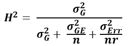
where

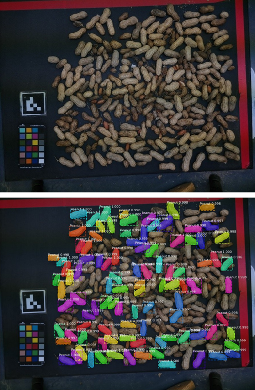
Figure 4. Example of Mask R-CNN input (top) and output (bottom) image on a field sample of the 2022 NCSU advanced yield trial. Each of the 100 detected pods is shown in a distinct color in the bottom image which represents their respective segmentation mask. All 100 detections are pods and no loose shelled kernel (LSK), stick, rock or other detritus were masked in a distinct color.

Results and Discussion

The imaging system as shown in Figure 1 costs $455 in total at the time of article submission (excluding tax and shipping). Assembly took approximately two hours once all components arrived. Software installation took approximately two hours for someone who is moderately familiar with computers.

The Mask R-CNN model accurately captured pod width data from images, achieving a precision of 0.99, recall of 0.94, F1 score of 0.96, and mAP@0.5 of 0.92. Spearman's correlation coefficients between the mechanical grade and Mask R-CNN model were 0.89, 0.89, and 0.93 (p-value = 2.2e-16) for No. 1, Fancy, and Jumbo pods respectively, indicating strong agreement across all three grade categories. Figure 3 shows the reduction in the loss function across training and validation datasets across all 50 epochs. The reduction in loss function means the model is getting better at its task by making fewer and smaller errors during training. More specifically in this situation, the model is getting better at correctly identifying pods and drawing accurate pixel-level masks around them. As seen in the right panel of Figure 3, beyond a certain number of epochs the model began to overfit the training data, evidenced by a marked increase in validation loss despite continued reductions in training loss, confirming that checkpoint selection was necessary to identify the best performing model. As shown in Figure 4, the model successfully differentiated peanut pods from loose shelled kernels (LSKs), rocks, sticks, and other detritus, with each of the 100 detections shown in a distinct color.

As expected, pod width data was normally distributed within each pod class (Figure 5). Small-podded breeding lines peak around 10-11 mm in width with nearly all pods falling below 14 mm and into the blue, No.1 pan. Medium-podded breeding lines peak around 15-16 mm, straddling the boundary between the white fancy bin and the red jumbo bin. Large-podded lines peak around 18 mm but range in width from 14-22 mm. While small-podded lines can be easily distinguished from the medium-podded lines by the pod roller, there is considerable overlap between the medium-podded and large-podded lines. This indicates the pod roller may not be able to perfectly distinguish between these two classes.

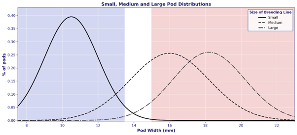
Figure 5. Examples of pod width (mm) distribution outputs from the MRCNN model from known large, medium, and small podded NCSU breeding lines. Blue background represents the No. 1 bin, white background the Fancy bin, and red background represents the Jumbo bin as defined by USDA regulations. As expected, pod width was normally distributed within each pod class.

Modeling showed significant effects from environment, block-by-environment and genotype, with genotype being by far the most significant (Table 1). This is desirable for the breeder as it means that selection for a desired pod size based on genotype should be highly effective and that varieties should perform reasonably similar across different environments. Within Table 1, Log Likelihood measures how well the model fits the data when that factor is included and is the basis for calculating the remaining columns. The Likelihood-Ratio Test (LRT) is the key test statistic here as it compares the log likelihood of a model with the factor included versus without. A larger LRT means removing the factor causes a bigger drop in model fit, indicating that the factor explains more of the variation in pod width. The LRT of genotype dwarfs the other three confirming it is the most important driver of pod width studied. P-value reports the probability of observing the reported LRT by random chance if the factor had no actual effect on pod width.

Table 1

– Analysis of Variance (ANOVA) output from the pod width linear mixed-effect model generated using the ranova() function of R’s lme4 package. Degrees of freedom for all factors was 1. This shows significant effects on pod width from block x environment, environment, and genotype, with genotype being the most significant.

Broad sense heritability for pod width was calculated as 0.81. This high value was expected as it has been previously reported that pod traits exhibited high heritability in a bi-parental mapping population containing the NCSU breeding line NC 3033 (Chavarro et al, 2020). The high heritability shown here suggests these traits are controlled by a small number of genes, each with strong effects that are relatively stable across environments (Bernardo, 2010). This implies pod width would be particularly amenable to marker-assisted selection once suitable markers have been developed. Towards this end, we plan to conduct a genome-wide association study (GWAS) on the 265 lines phenotyped in this study and have developed two bi-parental mapping populations segregating for pod width for phenotyping and genotyping.

While this study provides a solid foundation for modernizing peanut grading, several avenues for future research emerge. First, mounting the camera directly on the mechanical pod roller allows the grade to be taken while pre-sizing the pods for shelling, further increasing the speed and efficiency of the operation. Then, a second camera can be installed to capture images or video of seeds as they exit the sheller, thereby modernizing the seed grading process as well. Additionally, the MRCNN models could be retrained on a lighter weight framework allowing them to run on the cameras themselves, reducing computing time and power required. Finally, this second camera could be used to count peanut seeds at scale, enabling the sale of peanut seed by count instead of weight to farmers. Future work may also explore the use of depth imaging at sufficient distances and resolutions to be able to capture another pod trait. All data and code for this project is available at https://github.com/nkgarrity/Peanut-Pod-MRCNN.

Summary and Conclusions

This study demonstrated the successful integration of advanced computer vision-based phenotyping to quantify pod width, the sole determinant of pod grade. The MRCNN model achieved a precision score of 0.99, a recall score of 0.94, an F1 score of 0.96 and a mAP50 of 0.92 exhibiting strong ability to recognize peanut pods. The pod characterization between the mechanical grade and the MRCNN system showed Spearman’s correlation coefficients of 0.89 for the No1 category, 0.89 for the Fancy category and 0.93 for the Jumbo category. The system is simple, affordable, and specifically designed for use by breeding programs, academic labs, farmers, extension agents, and agronomists to estimate prospective grade prior to obtaining an official grade.

The authors would like to thank the North Carolina Peanut Growers Association for their financial support of this project.

Literature Cited

Abdulla W. 2017. Mask R-CNN for object detection and instance segmentation on Keras and TensorFlow (Version 2.1) [Computer software]. GitHub. https://github.com/matterport/Mask_RCNN.

Afonso M., Fonteijn H., Fiorentin F. S., Lensink D., Mooij M., Faber N., Polder G., and Wehrens R. 2020. Tomato fruit detection and counting in greenhouses using deep learning. Frontiers in Plant Sci. 11: 571299.

Anaconda Inc. ( 2023). Anaconda [Computer software]. https://www.anaconda.com/.

Bates D., Mächler M., Bolker B., and Walker S. 2015. Fitting linear mixed-effects models using lme4. J. Statistical Software. 67(1):1–48. doi: [: 10.18637/jss.v067.i01].

Bernardo R. 2010. Breeding for quantitative traits in plants 2nd ed.Stemma Press.

Bradski G. 2000. The OpenCV library. Dr. Dobb's Journal: Software Tools for the Professional Programmer. 25(11): 120–123.

Chavarro C., Chu Y., Holbrook C., Isleib T., Bertioli D., Hovav R., Butts C., Lamb M., Sorensen R., and Jackson S. 2020. Pod and seed trait QTL identification to assist breeding for peanut market preferences. G3: Genes, Genomes, Genetics. 10(7): 2297–2315.

Dickens J. W. 1962. Shelling equipment for samples of peanuts (Marketing Research Report No. 528). U.S. Department of Agriculture, Agricultural Marketing Service, Market Quality Research Division.

Garrido-Jurado S., Muñoz-Salinas R., Madrid-Cuevas F. J., and Marín-Jiménez M. J. 2014. Automatic generation and detection of highly reliable fiducial markers under occlusion. Pattern Recognition. 47(6): 2280–2292.

Google . 2021. TensorFlow (Version 2.5.0) [Computer software]. Python Package Index. https://pypi.org/project/tensorflow/2.5.0/.

Google . 2023. Google Colaboratory [Cloud-based computing environment]. https://colab.research.google.com/.

Hafiz A. M., and Bhat G. M. 2020. A survey on instance segmentation: State of the art. International Journal of Multimedia Information Retrieval. 9(3): 171–189.

Harris C. R., Millman K. J., Van Der Walt S. J., Gommers R., Virtanen P., Cournapeau D., Wieser E., Taylor J., Berg S., and Smith N. J. 2020. Array programming with NumPy. Nature. 585(7825): 357–362.

Hasty.ai. 2023. Hasty.ai [Image annotation software]. https://hasty.ai/.

He K., Gkioxari G., Dollár P., and Girshick R. 2017. Mask R-CNN. In Proceedings of the IEEE International Conference on Computer Vision (ICCV) (pp. 2961–2969). doi: [: 10.1109/ICCV.2017.322].

Isleib T. G., Wilson R. F., and Novitzky W. P. ( 2006). Partial dominance, pleiotropism, and epistasis in the inheritance of the high-oleate trait in peanut. Crop Sci. 46(3): 1331–1335.

Jordan D. L. 2023. 2023 peanut information. NC State Extension Publications. https://content.ces.ncsu.edu/peanut-information.

Lin T. Y., Maire M., Belongie S., Hays J., Perona P., Ramanan D., and Zitnick C. L. 2014. Microsoft COCO: Common objects in context. European Conference on Computer Vision (pp. 740–755). Springer International Publishing.

Luxonis . 2023. DepthAI Python Library (Version 2) [Computer software]. https://github.com/luxonis/depthai-python.

McKinney W. 2011. pandas: A foundational Python library for data analysis and statistics. Python for High Performance and Scientific Computing. 14(9): 1–9.

Spearman C. 1904. The proof and measurement of association between two things. The American J. Psychology. 15(1): 72–101. doi: [: 10.2307/1412159].

Stalker H. T. 1997. Peanut (Arachis hypogaea L.). Field Crops Res. 53(1–3): 205–217.

TensorFlow Developers. 2023. TensorBoard [Computer software]. GitHub. https://github.com/tensorflow/tensorboard.

Toda Y., Okura F., Ito J., Okada S., Kinoshita T., Tsuji H., and Saisho D. 2020. Training instance segmentation neural network with synthetic datasets for crop seed phenotyping. Communications Biology. 3(1): 173.

United States Department of Agriculture, Agricultural Marketing Service. 2019. Farmers' stock peanuts inspection instructions. Specialty Crops Inspection Division. https://www.ams.usda.gov/grades-standards/farmers-stock-peanut-inspection-instructions.

United States Department of Agriculture. 2025. Peanut prices. National Agricultural Statistics Service, Agricultural Statistics Board.

Vladimirov L. 2021. TensorFlow object detection API tutorial. Read the Docs. https://tensorflow-object-detection-api-tutorial.readthedocs.io/en/latest/.

Yang S., Zheng L., He P., Wu T., Sun S., and Wang M. ( 2021). High-throughput soybean seeds phenotyping with convolutional neural networks and transfer learning. Plant Methods. 17(1): 50.