Introduction
As a natural process related to harvesting, handling, and curing, farmers' stock (FS) peanuts may contain a variety of foreign material (FM) such as dirt, sticks, rocks, grain seeds, metal objects, and glass (Davidson et al., 1982). Once shellers purchase FS peanuts from the farmer, they try to remove as much of the FM as possible using a variety of methods when moving peanuts into and out of storage facilities and during the shelling process (Davidson et al., 1982). The goal of the sheller is to remove as much of the FM as economically and technically possible. Since foreign material in the finished or processed nuts can be a hazard to consumers and an economic liability, food manufacturers have put increasing pressure on shellers to approach 100% FM removal so that little to no FM remains in shelled peanut lots when shipped to a food manufacturer.
Food manufacturers may specify that FM in a lot provided by a sheller not exceed a maximum limit or maximum concentration. Foreign material concentration may be expressed as the number of FM pieces per unit mass of peanuts or the maximum number of FM pieces in the entire lot. For example, the food manufacturer may specify that lots should not contain more that one piece of FM per 2000 pounds of peanuts. With food manufacturers specifying lower and lower limits for FM, shellers have two problems: (1) having the resources and/or technology to remove FM so that shelled lots do not exceed maximum limits specified by the food manufacturers and (2) how to accurately estimate the true level of FM in a processed lot to determine if contract specifications have been met. The sheller measures the FM in a lot at origin and the food manufacturer may measure the FM at destination to determine if the sheller has met contract specification. This paper will deal only with the second issue of how to get an accurate estimate of the true level of FM in the lot.
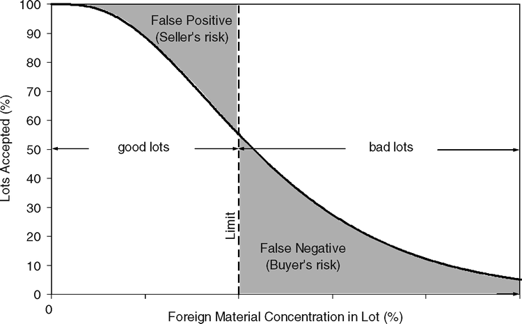
The sheller and food manufacturer estimate the FM contamination in the bulk lot by taking one or more samples from the lot and counting the number of FM pieces in a sample of a given mass. Because the number of FM pieces among replicate samples taken from the same lots will differ, the sheller can never determine the true proportion of FM in the lot with 100% confidence. Because of the variability among sample test results, some lots will be misclassified. There is a chance that samples from a good lot will test bad (false positive or seller's risk). There is a chance that samples from bad lots will test good (false negative or buyer's risk). It is important for the food manufacturer and sheller to know the effect of sample size (or number of samples of a given size) on the uncertainty associated with using samples to estimate the true proportion of FM a lot and how to reduce misclassification of lots relative to a limit specified by the food manufacturer.
The objectives of this study were to (1) measure the variability and FM distribution among sample test results when estimating the true lot proportion of FM in a lot of shelled peanuts, (2) compare the measured variability and FM distribution among sample test results to that predicted by the binomial distribution, (3) develop a computer model, based upon the binomial distribution, to evaluate the performance (buyer's risk and seller's risk) of sampling plan designs used to estimate FM in a bulk lot of shelled peanuts, and (4) demonstrate with the model the effect of increasing sample size to reduce misclassification of lots.
Methods
Experimental
With the assistance of a peanut sheller in the southeastern U.S., 6 lots of shelled medium runner peanuts were identified for sampling to estimate the percent FM in each lot. Each lot was about 20 metric tonnes or about 45,400 pounds. Shelled medium runner peanut grades, defined by the Southeastern Peanut Association, are peanuts that are milled through a screen having 8.3 mm × 19.1 mm (21/64 by ¾ inch) openings and which will either meet an average of 40 to 50 count per ounce or which will pass through a screen having 7.1 mm × 19.1 mm (18/64 by ¾ inch) openings. A total of 88 samples, 9 kg (about 20 pounds) each, were taken from each lot. Using a scooping device, the 9 kg samples were taken at even intervals (about every 500 pounds) from the beginning to the end of the lot. Each 9 kg sample was identified with a lot number and sample number. Personnel from the Federal State Inspection Service weighed each sample, removed FM from each sample, and counted the total number of FM pieces (N) in each sample. The number of kernels in the 9 kg sample (n) was not counted, but estimated by multiplying the sample mass times the mean count per unit mass (industry standard of 1584 per kg (45 per oz) for shelled medium runner peanuts). The percent FM (PFM) for each sample was calculated by dividing the number of FM pieces (N) by the number of kernels (n) in the sample (N/n) and multiplying by 100. The lot number, sample number, sample weight, number of FM pieces, and percent FM was recorded in a database. The mean, m, and variance, s2, among the 88-sample test results for PFM was computed for each lot.
Theoretical Considerations
It was assumed that a peanut lot consisted only two types of objects, a peanut kernel and a piece of FM and the FM had physical characteristics similar to a peanut. The last assumption may be valid because any FM that remains in the lot after all shelling operations is probably very similar in physical characteristics to a peanut kernel or the FM piece would have been removed. It was assumed that the variance and FM distribution among the 88-sample test result per lot could be described by the binomial distribution (Whitney, 1961). The binomial distribution is a discrete distribution where the outcome is either success or failure. For example, an object in the lot is either a peanut or a piece of FM.
From the binomial function, the probability of obtaining exactly k successes (k pieces of FM) in a sample of n kernels taken from a lot with a true proportion of FM pieces of p is described by Equation 1.
 (1)
(1)
If a sample test result is expressed as the number of FM pieces (N), then average (μ) among replicate sample test result of n peanuts is n times p or np if the true proportion of FM pieces in the lot is p. The variance σ2 among replicate sample test results of n peanuts is np(1-p). If the number of FM pieces is expressed as a percent of the total number of peanuts in the sample (PFM = 100N/n), the mean and variance is described by equations 2 and 3, respectively.
 (2)
(2)
 (3)
(3)
From equation 3, it can be seen that the variance is a quadratic function of the mean μ. As p increases from 0 to 50%, the variance increases. As p continues to increase from 50 to 100%, the variance decreases. At p = 0 and 100%, the variance is zero and at p = 50%, that variance is a maximum.
The mean μ, variance σ2, and distribution among sample test results predicted by the binomial distribution were compared to the experimentally measured mean m, variance s2, and observed distribution among the 88-sample test results for each lot when the sample test result is expressed percent FM pieces (PFM). The comparisons were made to determine if the binomial function can be used to accurately predict the effect of sample size on the variability and distribution among sample test results. From the distribution of sample test results, the effect of sample size on the buyer's risk and seller's risk can be predicted (Whitaker, 2006; Whitaker, et al., 2007).
Results
The number of samples, average sample size in grams (g) and number of kernels (n), the sum of the number of FM pieces (ΣN) among all samples for each lot, and the estimated true proportion of FM pieces in each lot (p) is shown in Table 1. While 88 nine kilograms (20 lbs) samples were the target values, the actual number of samples and size sample varied slightly from lot to lot (Table 1). The true proportion of FM pieces in the lot (p) was calculated by dividing the sum of the FM pieces (ΣN) by the estimated sum of the number kernels (Σn) in all samples taken from each lot. Sample size in number of kernels (n) was estimated by multiplying the sample mass times the mean count per kg of 1586 (45 kernels per once). The lots are ranked in Table 1 by the estimated true proportion of FM pieces (p) in the lot.
The frequency distribution or the number of samples that contained 0, 1, or 2 pieces of foreign material is shown in Table 2. No sample from any of the six lots contained more than 2 pieces of foreign material. From the estimated true proportion of FM pieces (p) in a lot (Table 1), the calculated total number of FM pieces in the six lots ranged from 23 FM pieces (lot 1) to 172 FM pieces (lot 6) per 45,400 pounds or 1 FM piece per 1,913 lbs (lot 1) to 1 FM piece per 255 lb (lot 6). It is understandable that a 20 lb sample would miss the FM and such a high percentage of all samples taken from a lot would have zero FM pieces.
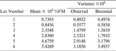
Table 3 shows the observed mean and variance among sample test results for each of the six lots when the sample test result is expressed PFM (100N/n), and variance predicted by the binomial function (Equation 3). The variances are ranked in Table 3 by the mean PFM in ascending order. The observed variances are of similar magnitude to the variances predicted by the binomial function (except lot 4) and increase with mean PFM as predicted by the binomial distribution. With the exception of lot 4, the percent difference between variances range from 1.0% (lot1) to 8.8% (lot 6). The large deviation (41.2%) between the observed and predicted variances that occurred in lot 4 can't be explained.
Another way to judge the suitability of the binomial distribution is to compare the observed cumulative distribution among sample test results (constructed from Table 2) to the cumulative distribution predicted by the binomial distribution for each lot (Equation 1). The observed and predicted cumulative distributions showing the probability of obtaining a sample with at least 0, 1, or 2 FM pieces for lot 4 is shown in Table 4. The cumulative probability distribution among sample test results for lot 4 reflects a sample size of 15826 kernels and a true proportion of FM (p) in the lot of 2.838 × 10⁻⁶.
The Kolmogorov-Smirnov (K-S) goodness of fit (GOF) test was used to determine with 95% confidence if the observed distribution could have been sampled from a binomial distribution (Benjamin and Cornell, 1970). The K-S test compares the absolute maximum difference in the cumulative probabilities (Dmax) between the observed and predicted distributions to a critical difference (Dcritical) value for 95% confidence limits (cl) and number of samples in the observed distribution (86 for lot 4). If |Dmax| < = Dcritical, the null hypothesis that the observed distribution was sampled from a binomial population can't be rejected with 95% confidence limits. In Table 4 Dmax is 0.03443 and Dcritical for 95% confidence limits and 86 samples is 0.147 (Dcritical = 1.36/√86). Since 0.0344 < = 0.147, the null hypothesis that the observed distribution was sampled from a binomial distribution can't be rejected at the 95% confidence level. The Dmax for the observed and predicted cumulative distributions for all six lots is shown in Table 5 along with the Dcritical value for 95% cl. The value of Dcritical varies slightly because the number of samples taken from each lot varies from lot to lot. As Table 5 indicates, the null hypothesis can't be rejected at the 95% confidence level for any of the six lots since Dmax < = Dcritical for all lots (Table 5).
Maximum difference (Dmax) between the observed and predicted cumulative distributions and the critical difference (Dcritical) for 95% confidence limits and number of samples in the observed distribution. If Dmax < = Dcritical, then the null hypothesis that the observed distribution was sampled from a binomial distribution can't be rejected with 95% confidence limits.
Operating Characteristic Curves
An operating characteristic (OC) curve can be used to describe the performance of a sampling plan design given the sample size, n, and a foreign material accept/reject limit, fma. The accept/reject limit is usually equal to (but not required to be equal to) a defined foreign material tolerance, fmt. The seller of the lot may choose to use an accept/reject limit that differs from a tolerance specified by the buyer. Because of the variability among sample test results, there is a certain probability that a lot with a true PFM will be accepted or rejected (reject = 1.0 − accept) when measuring the foreign material, fm, in a sample. The fm in the sample is compared to the accept/reject limit fma and the lot is accepted or rejected depending on whether fm < = fma or fm > fma, respectively. A plot of the accept probability versus the true PFM (100p) in the lot is called an OC curve. A generalized OC curve is shown in Figure 1.
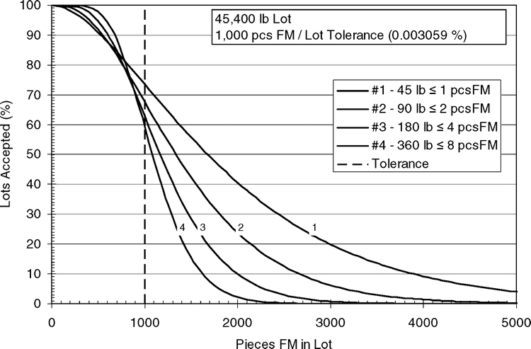
The binomial distribution can be used to predict the accept probabilities (OC curve) for a given sample size (n), accept/reject limit, fma when sampling a lot with a true PFM. The effect of sample size, accept/reject limit, and multiple samples on the buyer's risk and seller's risk are shown below using OC curves. All examples are for US medium runner lots (45 kernels per ounce) and a maximum limit specified by the buyer that the lot should not contain more than 1000 foreign material pieces in the entire lot (45,400 lb) of peanuts or a ratio of 1 FM piece per 45.4 lbs. Since the number of kernels in the lot is 32,688,000, the maximum limit (fmt) is equal to (1000/32,688,000)100 or 3.0592 × 10⁻³%.
Sample Size
The effect of increasing sample size from 45 to 90 to 180 to 360 pounds and using accept/reject limits of 1, 2, 4, and 8 FM pieces (PFM = 3.0592 × 10⁻³ %) is shown in Figure 2. The maximum limit of 1000 FM pieces in a 45,400 lb lot is the same ratio as 1, 2, 4, or 8 FM pieces in 45, 90, 180, and 360 pound (45 kernels per ounce) samples, respectively. As sample size increases, the OC curve gets steeper. The probability of accepting good lots (lots with less than 1000 FM pieces) increases with sample size and the probability of accepting bad lots (lots with more than 1000 FM pieces) decreases. Increasing sample size decreases both the buyer's risk and the seller's risk. For example, a lot with 2000 FM pieces will be accepted 40, 25, 10, and 2% of the time (point estimate of the buyer's risk) when using a 45, 90, 180, and 360 pound sample, respectively.
Accept/reject Limit
In the above example showing the effect of sample size (Figure 2), the accept/reject limit (expressed as a percent FM) was held constant and equal to the maximum limit of 1000 FM pieces in the entire lot (PFM = 3.0592 × 10⁻³ %). In Figure 3, the effect of reducing the accept/reject limit relative to the maximum limit is shown for a constant sample size of 180 pounds. The effect of using four accept/reject limits 4, 2, 1, and 0 FM pieces (PFM = 3.0592 × 10⁻³, 1.5432 × 10⁻³, 0.7716 × 10⁻³, and 0.0 %) on the accept and reject probabilities (OC curve) are shown in Figure 3. As the accept/reject limit decreases, the OC curve shifts to the left and the accept probabilities decrease for all lot PFM levels. For example, the probability of accepting a lot with 1000 FM pieces when using an accept/reject limit of 4, 2, 1, and 0 FM pieces are 63, 24, 9, and 2 %, respectively. If a sheller wanted a sampling plan that would accept 5% or less of the lots with 1000 or more FM pieces, he would have to use an accept/reject limit of 0 FM pieces when using an 180 lb sample. If 1 or more FM pieces were found in the sample, the lot should be rejected.
Reducing the accept/reject limit relative to the maximum limit reduces the bad lots accepted or buyer's risk. However, reducing the accept/reject limit relative to the maximum limit also increases the good lots rejected or the seller's risk. For example, the probability of accepting a lot with 500 FM pieces when using an accept/reject limit of 4, 2, 1, and 0 FM pieces are 95, 70, 40, and 14 %, respectively. When using an accept/rejct limit lower than the maximum limit specified by the buyer, the seller runs a higher risk of rejecting good lots in order to reduce the risk of accepting bad lots.
The performance of four sampling plans that use accept/reject limits of 4, 2, 1, and 0 foreign material pieces to accept or reject a lot when the buyer has specified that the lots must not contain more than a total of 1000 foreign material pieces. All four sampling plans use a constant sample size of 180 pounds.
Multiple Samples
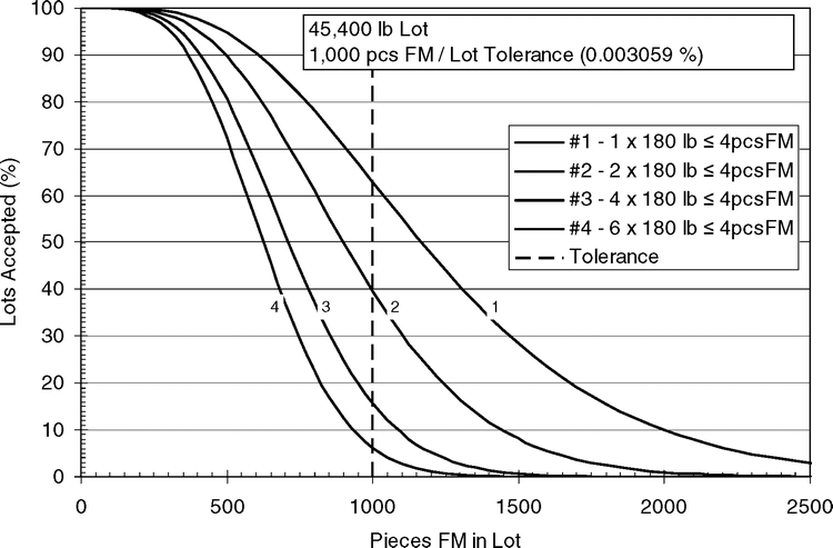
The effect of taking multiple samples from a lot and averaging all sample test results is the same as increasing sample size (Figure 2). However, if all sample test results have to be less than or equal to an accept/reject limit, the performance is very different from averaging sample test results. The effect of requiring 1, 2, 4, and 6 180 lb samples to all test less than or equal to 4 FM pieces is shown in Figure 4. As the number of samples required to test less than or equal to the accept/reject limit increases, the OC curves shift to the left and the accept probabilities decrease for all lot FM concentration. The effect is similar to that shown in Figure 3 when reducing the accept/reject limit relative to a maximum limit. Requiring all the sample test results to test less than or equal to the accept/reject limit decreases the bad lots accepted (buyer's risk), but increases the good lots rejected (seller's risk).
Performance of four sampling plans that require 1, 2, 4, and 6 180 lb samples to all test less than or equal to the accept/reject limit of 4 foreign material pieces (Percent foreign material = 3.0592 × 10⁻³). Maximum limit allowed by the buyer is a total of 1000 foreign material pieces in the entire lot.
As buyers specify lower maximum limits for total FM pieces in the lot, sample size will have to get larger and/or accept/reject limits much smaller than the maximum limit will have to be used to meet specified risk levels. At some point using samples to determine if a lot meets specifications becomes prohibitive. For example, specifying maximum limits of 1000, 100, and 10 FM pieces in a 45,400 lb lot requires a minimum sample size of 45.4, 454, and 4,540 lb, respectively, with an accept/reject limit of 1 FM piece. At low maximum limits, the handler will require electronic sorters to reliably remove FM from the lots with an efficiency approaching 100%.
The binomial distribution can also be applied to designing sampling plans for attributes other than FM such as damaged kernels, kernels with biotech traits, and kernels with spots. An interactive program is available on the Internet where the performance of sampling plans can be calculated given the design parameters (Whitaker, 2006).
References Cited
Benjamin J. R. and Cornell C. A. 1970 Probability, statistics, and decision for civil engineers. McGraw-Hill New York, NY 466 – 475 .
Davidson J. I. , Whitaker T. B. , and Dickens J. W. 1982 Grading, cleaning, storage, shelling, and marketing of peanuts in the United States. 571 – 623 In Pattee H. E. and Young C. T. Peanut Science and Technology American Peanut Research and Education Society, Inc Yoakum, Texas .
Whitaker T. B. 2006 Operational Characteristic Curves. http://www5.bae.ncsu.edu/usda/www/ResearchActDocs/index.htm (last accessed May 13, 2008) .
Whitaker T. B. 2006 Sampling foods for mycotoxins, Food Additives and Contaminants. 23 : 50 – 61 .
Whitaker T. B. , Doko M. B. , Maestroni B. M. , Slate A. B. , and Ogunbanwo B. F. 2007 Evaluating the performance of sampling plans to detect fumonisin B1 in maize lots marketed in Nigeria. J. Assoc. Official Analytical Chemists, Int 90 : 1050 – 1059 .
Whitney D. R. 1961 Elements of mathematical statistics, Holt, Rinehart, and Winston, New York, NY. 32 – 35 .
Notes
- USDA, ARS, Box 7625, NC State University, Raleigh, NC 27695 [^]
- Biological and Agricultural Engineering Department, Box 7625, NC State University, Raleigh, NC 27695-7625 [^]
- Statistics Department (retired), Box 8203, NC State University, Raleigh, NC 27695-8203 [^]
Disclaimer
The use of trade names in this publication does not imply endorsement by the USDA or the N.C. Agricultural Research Service of the products named nor criticism of similar ones not mentioned.
Author Affiliations


